Virial Coefficients

We will focus on the B–coefficient here. The Virial module has been inspired by a paper by Reid in J. Chem. Educ. which was concerned with obtaining inter–molecular interaction potentials from the knowledge of the second virial coefficient [3]. Assuming pairwise inter–molecular interaction potentials that depend only on the distance r between two molecules (such as the LJ potential), one can show that the B coefficient can be obtained from a simple one–dimensional integration over the potential U(r) as follows:

$B(T) = -2\pi N_A \int_{0}^{\infty} dR \cdot R^2 [e^{-\frac{U(R)}{kT}} - 1]$ ..... (Equation 7a)

For the LJ potential of Eq. (3) the integration in Eq. (7) can be carried out analytically, with the result expressed in terms of the confluent hypergeometric function $_1F_1(a, b, z)$

$$B_{LJ}(T) = -\frac{\pi N_A}{3 \sqrt{2} (kT)^{3/4}} \left[\sqrt{kT} \Gamma\left(-\frac{1}{4}\right) \text{ }_1F_1\left(-\frac{1}{4},\frac{1}{2},\frac{1}{kT}\right)+2 \Gamma\left(\frac{1}{4}\right) \text{ }_1F_1\left(\frac{1}{4},\frac{3}{2},\frac{1}{kT}\right)\right]$$

where $\Gamma(x)$ is the gamma function.

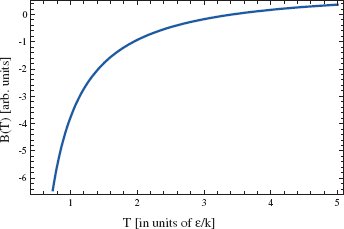
The qualitative behavior of B as a function of T based on the LJ potential is shown in the figure below:

The general shape of this curve is in agreement with the data shown by Reid [3] for Argon (see Fig. 1 in Ref. 3 which shows experimental data for Argon and a fit to a Maitland–Smith potential). In the presence of the quadrupole (Q) term, the potential U in Eq. (7) has additional terms from Q which can be added by considering an expansion of U(r) at large distances. The potential also becomes dependent on the relative orientation of the two molecules, which means the integral in (7) has additional angular–dependent terms. This leads to modifications of the magnitude of B and to the shape of the curve although the overall shape is qualitatively similar to the one shown in the figure above.

Specifically, the electrostatic energy of interaction of two point quadrupoles, each of magnitude Q is

$$U_{QQ}(r, \theta_A, \theta_B, \phi) = \frac{Q^2}{r^5} f(\theta_A, \theta_B, \phi)$$

where the orientation-dependent part $f(\theta_A, \theta_B, \phi)$ is defined

$f(\theta_A, \theta_B, \phi) = \frac{3}{4}[1 - 5 cos^2\theta_A - 5 cos^2\theta_B - 15 cos^2\theta_A cos^2\theta_B + 2(4 cos\theta_A cos\theta_B - sin\theta_A sin\theta_B cos\phi)^2]$

Accordingly, the formula for the virial coefficient in terms of the potential must be modified to include integration over the orientational coordinates, thus

$B(T) = -\frac{1}{4} N_A \int_{0}^{\infty} dR \cdot R^2 \int_{0}^{\pi} d\theta_A sin\theta_A \int_{0}^{\pi} d\theta_B sin\theta_B \int_{0}^{2\pi} d\phi [e^{-\frac{1}{kT}(U_{LJ}(R)+U_{QQ}(R,\theta_A, \theta_B, \phi))} - 1]$ ..... (Equation 7b)

This integral cannot be evaluated in a general way in terms of any standard functions. To proceed further, we consider a series expansion that is valid for small values of the quadrupole moment Q. To this end we expand the exponential of the quadrupole contribution,

$B(T) = \frac{1}{4} N_A \int_{0}^{\infty} dR \cdot R^2 \int_{0}^{\pi} d\theta_A sin\theta_A \int_{0}^{\pi} d\theta_B sin\theta_B \int_{0}^{2\pi} d\phi \left[1 - e^{-\frac{1}{kT}U_{LJ}(R)}\sum_{n=0}^{\infty}\frac{(-kT)^{-n}}{n!}(U_{QQ}(R,\theta_A, \theta_B, \phi))^n\right]$ ..... (Equation 7c)

which can be rearranged into the form

$B(T) = B_{LJ}(T) - \frac{1}{4} N_A \sum_{n=1}^{\infty}\frac{1}{n!}(-kT)^{-n}Q^{2n}\left[\int_{0}^{\infty} dR \cdot R^{2-5n} e^{-\frac{1}{kT}U_{LJ}(R)}\right]\left[\int_{0}^{\pi} d\theta_A sin\theta_A \int_{0}^{\pi} d\theta_B sin\theta_B \int_{0}^{2\pi} d\phi (f(\theta_A, \theta_B, \phi))^n\right]$ ..... (Equation 7d)

For any given n the orientational integrals resolve into a simple ratio, and the integral over separation can be expressed in terms of the confluent hypergeometric function. The general form of the result is

$$B(T) = B_{LJ}(T) + N_A\sum_{n=1}^{\infty}q_n t_n(T) Q^{2n}$$

where

$t_n(T) = (kT)^{-\frac{7n+9}{12}} \left[\sqrt{kT} \Gamma\left(\frac{5n-3}{12} \right) \text{ }_1F_1\left(\frac{5n-3}{12},\frac{1}{2},\frac{1}{kT} \right) + 2 \Gamma\left(\frac{5n+3}{12}\right) \text{ }_1F_1\left(\frac{5n+3}{12},\frac{3}{2},\frac{1}{kT}\right)\right]$

and the first few coefficients q_n are given in the following table.

n	qn
1	$0$
2	$-\frac{7\pi}{60\cdot2^{1/6}}$
3	$\frac{3\pi}{245}$
4	$-\frac{71\pi}{1960\cdot2^{5/6}}$
5	$\frac{16\pi\cdot2^{1/3}}{4235}$
6	$-\frac{18033\pi}{4580576\cdot2^{1/2}}$